Starting with Excel can feel overwhelming. You are looking at a massive grid of blank boxes, and it is hard to know where to begin. This beginner’s cheat sheet breaks down the absolute fundamentals. Learn the basic layout, the essential terminology, and the 5 everyday formulas that will make you look like a pro on day one.
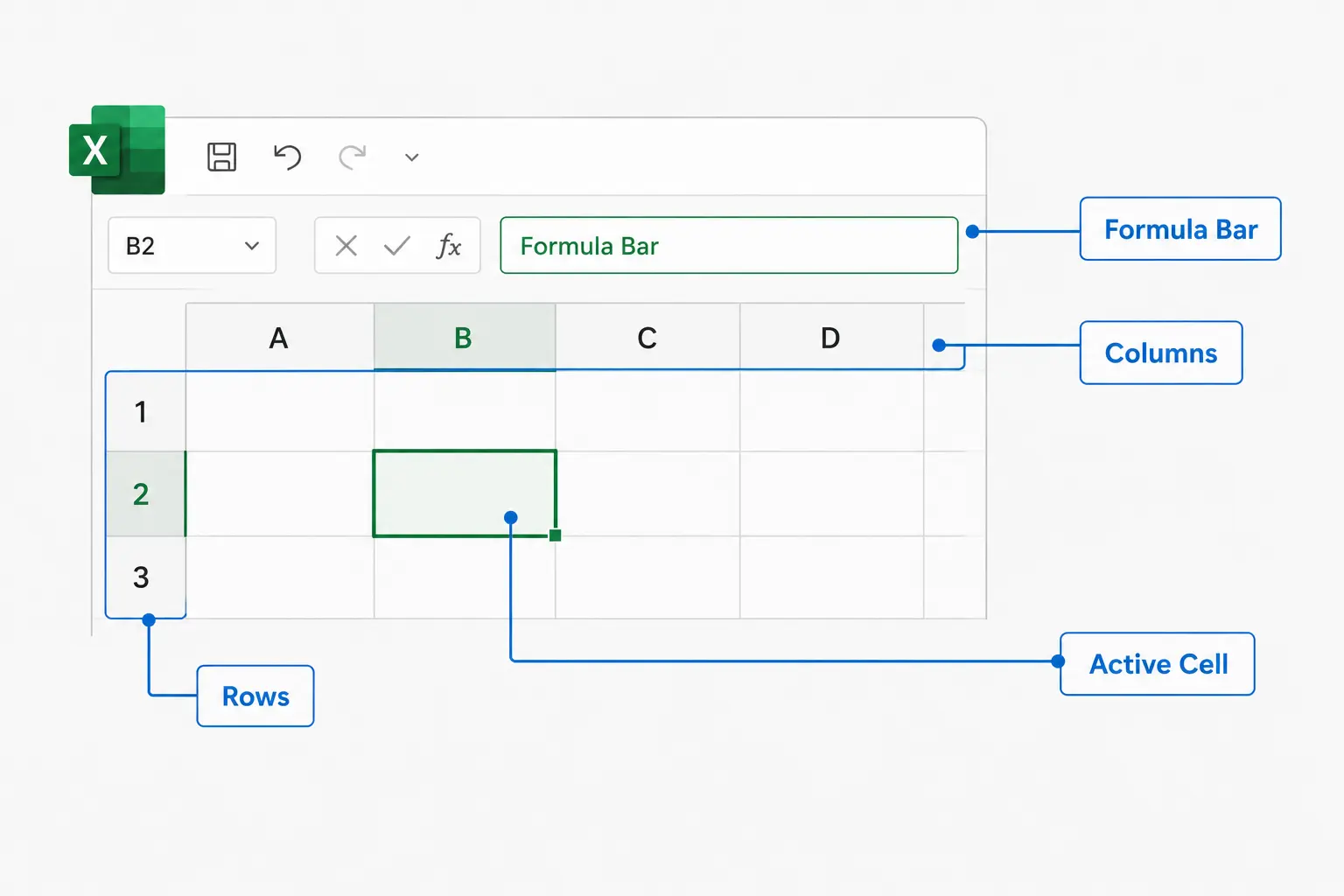
Figure: The basic anatomy of an Excel spreadsheet, highlighting columns, rows, the formula bar, and the active cell.
[BUTTON: Download Beginner Printable PDF]
1. The Anatomy of Excel: Basic Terms
Before writing formulas, you need to understand how Excel is structured. Think of it as a map with coordinates.
| Term | What it Means | Example / Visual |
|---|---|---|
| Workbook | The entire Excel file you open. It can hold multiple individual sheets. | Your saved file: Budget_2026.xlsx |
| Worksheet (Tab) | A single page inside your workbook. You switch between them at the bottom left. | “January Sales”, “Q2 Expenses” |
| Cell | A single box where rows and columns meet. Each cell has an address. | B4 (Column B, Row 4) |
| Formula Bar | The long white bar at the top of Excel. It shows what is actually inside a cell. | Displays =SUM(A1:A5) instead of the final number. |
| Range | A collection of two or more cells selected together. | A1:A10 (All cells from A1 down to A10) |
3. The 5 Basic Formulas Every Beginner Must Know
All Excel formulas begin with an equals sign (=). If you do not type =, Excel will just treat your formula as normal text.
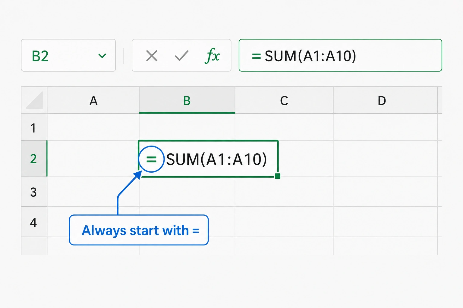
Figure: The golden rule of Excel formulas—always begin your syntax with an equals sign (=) to activate the function.
1. SUM (Add numbers together)
Instead of typing =A1+A2+A3, use SUM to add an entire range.
- How to type it:
=SUM(B2:B10) - What it does: Adds every single number between cell B2 and B10.
2. AVERAGE (Find the middle ground)
Calculates the mathematical mean of your selected numbers.
- How to type it:
=AVERAGE(C2:C20) - What it does: Adds the numbers and divides by the total count automatically.
3. COUNT (Count cells with numbers)
Tells you how many items are in your list, ignoring blank boxes or text.
- How to type it:
=COUNT(A2:A100) - What it does: Gives you a quick tally of how many entries have numeric data.
4. MAX & MIN (Find the highest and lowest)
Locates the biggest or smallest number in a dataset instantly.
- How to type it:
=MAX(D2:D50)or=MIN(D2:D50) - What it does: Great for finding the highest sales figure or lowest expense.
4. Golden Rules for Excel Beginners
- Keep Headers Simple: Use row 1 for your column titles (like Date, Name, Amount). Keep them bold and short.
- Never Mix Text and Numbers: If you write “10 USD” in a cell, Excel will treat it entirely as text and your formulas will fail. Write the number “10” alone, and format the column to currency instead.
5. Conditional Math & Counting (SUMIF & COUNTIF)
Standard formulas calculate everything in a range. Conditional formulas allow you to add or count data only if a specific rule or criteria is met.
1. SUMIF (Add data based on a rule)
Sums the values in a range that meet the criteria you specify. Perfect for isolating specific costs or sales categories.
=SUMIF(range, criteria, [sum_range])=SUMIF(B2:B20, "Software", C2:C20)What it does: Scans column B for the word “Software” and sums up the corresponding costs from column C.
2. COUNTIF (Count cells based on a rule)
Counts the number of cells within a range that match your single condition. Great for tracking completions, regions, or specific items.
=COUNTIF(range, criteria)=COUNTIF(D2:D50, "Completed")What it does: Tally up exactly how many times the status “Completed” appears in column D.
6. Text Manipulation & Cleaning (CONCAT, UPPER, LOWER, TRIM)
Data imported into Excel is rarely clean. These simple text functions allow you to combine strings, fix broken capitalization, and remove accidental spaces instantly.
1. CONCAT / CONCATENATE (Join text together)
Combines text from multiple cells into one single cell. Remember to manually add a space " " between strings if you are joining names!
=CONCAT(text1, text2, ...)=CONCAT(A2, " ", B2)What it does: Combines a first name in cell A2 and a last name in cell B2, separated by a clean space.
2. UPPER & LOWER (Fix broken case formatting)
Forces all text inside a selected cell to become either entirely UPPERCASE or entirely lowercase. Excellent for normalizing messy database inputs.
=UPPER(text) or =LOWER(text)=LOWER(C2)What it does: Converts a raw email address in cell C2 (like “John.DOe@EXAMple.com”) into perfect lowercase.
3. TRIM (Remove ghost spaces)
Strips away all extra spaces from a text string, leaving only single spaces between words. This fixes the hidden spaces that frequently break VLOOKUP and XLOOKUP formulas.
=TRIM(text)=TRIM(A2)What it does: Removes accidental double spaces or trailing spaces at the absolute end of cell A2.